Structured Neurons

In the previous demonstrations we considered point neuron models. However, biological neurons often posses elaborate dendritic trees, which allow them to pre-process the synaptic inputs before they reach the somatic spike initiation zone near the axon initial segment. Taking dendrites as well as their passive and active properties into account can greatly enhance the computational power of neurons [1-3].

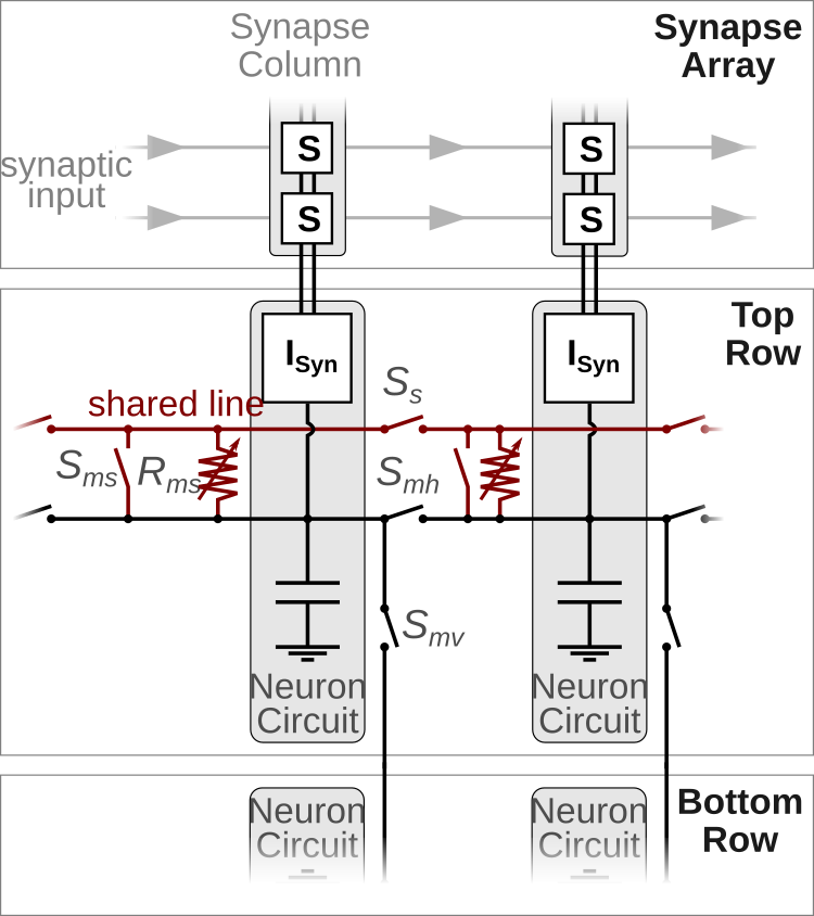
In order to investigate the features of structured neurons, BrainScaleS-2 offers the possibility to connect several neuron circuits to form multi-compartmental neuron models. The following figure shows a sketch of two neuron circuits and the electronic (not synaptic) connections they can establish.

Horizontal switches \(S_{mh}\) and vertical switches \(S_{mv}\) allow to connect neighboring neuron circuits directly – they form a single, isopotential compartment. This can be useful to increase the fan-in of a single compartment as it is now connected to several columns of the synapse array or might be needed to realize certain multi-compartmental models (see the code example below).

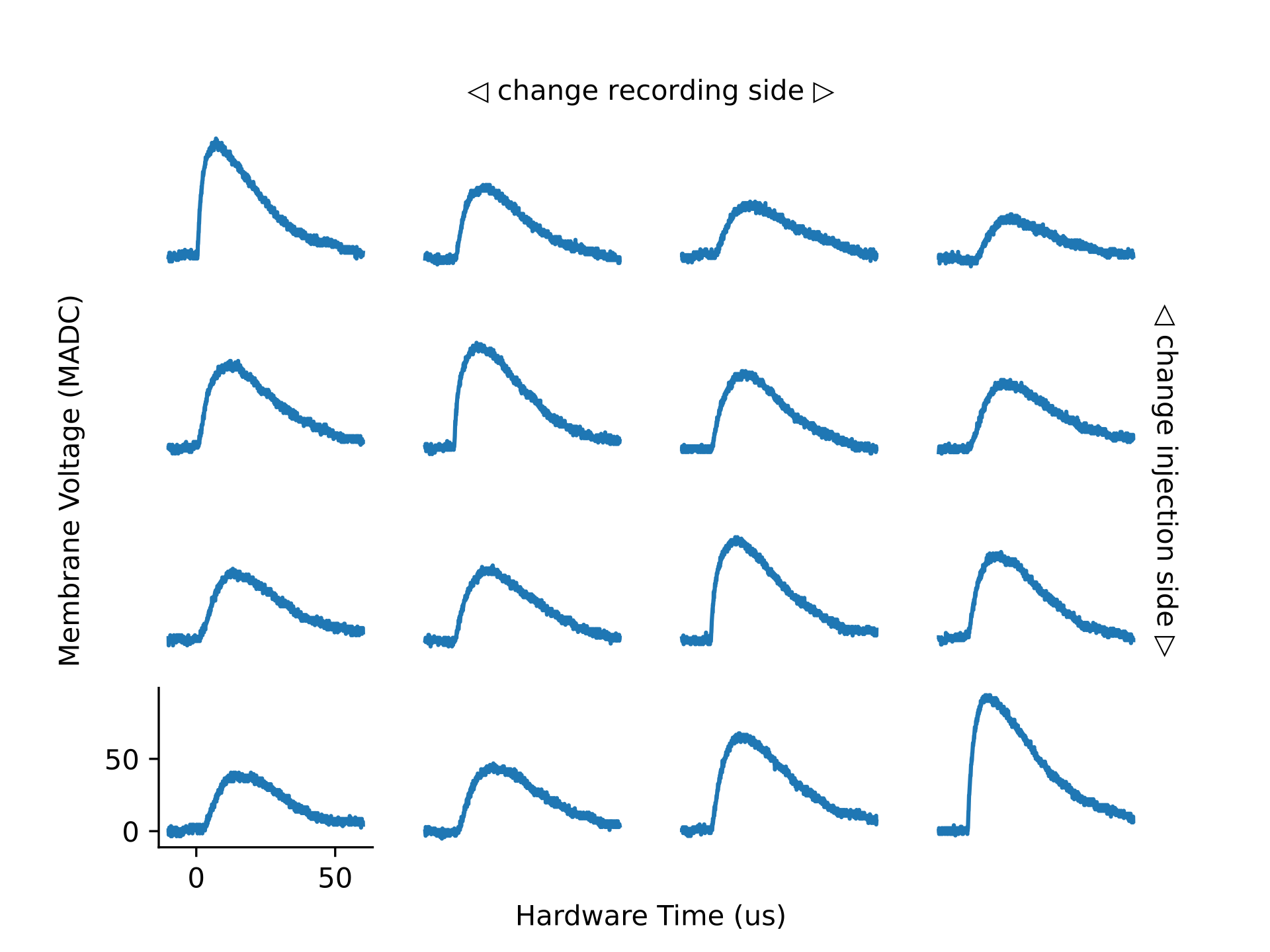
In addition to these “membrane connections” each neuron circuit can also connect either directly (\(S_{ms}\)) or via a conductance \(R_{ms}\) to a “shared line”. This offers the possibility to connect several compartments via conductances and to form various multi-compartmental neuron models. multi We will demonstrate the implementation of a multi-compartmental model by the example of a compartment chain and will investigate how excitatory postsynaptic potentials propagate along the chain. The following figure displays a sketch of a chain with four compartments in the top part; in the bottom the hardware implementation is illustrated.

The rest of this demo will motivate why we chose this hardware implementation and will show how this model can be emulated on the BrainScaleS-2 system. You can find more detailed information about the multi-compartmental capabilities, example configurations and experiments with structured neurons in Kaiser et al. 2021 [4].

References for further reading

1. Poirazi, P., Brannon, T., Mel, B.W., 2003. Pyramidal neuron as two-layer neural network. Neuron 37, 989–999. doi:10.1016/s0896-6273(03)00149-1

2. London, M., Häusser, M., 2005. Dendritic computation. Annu. Rev. Neurosci. 28, 503–532. doi:10.1146/annurev.neuro.28.061604.135703

3. Major, G., Larkum, M.E., Schiller, J., 2013. Active properties of neocortical pyramidal neuron dendrites. Annual Review of Neuroscience 36, 1–24. doi:10.1146/annurev-neuro-062111-150343

4. Kaiser, J., Billaudelle, S., Müller, E., Tetzlaff, C., Schemmel, J., and Schmitt, S., 2021. Emulating dendritic computing paradigms on analog neuromorphic hardware. Neuroscience. doi:10.1016/j.neuroscience.2021.08.013

Imports and Calibration

Once again we have to set some environment variables for our microscheduler first:

from _static.common.helpers import setup_hardware_client
setup_hardware_client()

We continue by importing several Python packages, which we need to perform our experiment.

%matplotlib inline
from functools import partial
from typing import List
import numpy as np
import ipywidgets as widget
import matplotlib.pyplot as plt
import quantities as pq

import pynn_brainscales.brainscales2 as pynn

A default calibration is generated for every setup every night. We save the nightly calibration in two variables such that we can use it later when we define our neuronal network.

from _static.common.helpers import get_nightly_calibration
calib = get_nightly_calibration()

Now we can start setting up our network:

# setup PyNN and inject calibration data
pynn.setup(initial_config=calib)

Furthermore, we define some global parameters which we need for the construction of the chain and the external stimulus.

length = 4  # Number of compartments in the chain
inputs = 10 # Number of concurrent input spikes

Constructing a Compartment Chain

The HXNeuron allows to set all relevant parameters of the BrainScaleS-2 neuron circuits. It particularly allows to control the direct connections between neuron circuits and the connections to the somatic line.

We will now create a chain of compartments, which are connected via conductances. Each compartment in the middle of the chain has two neighbors. Therefore, these compartments have to establish two connections via the somatic line. As a consequence each is made up of two neuron circuits: the first will connect to the somatic line via the conductance and the second via the switch.

In order to form the chain with length compartments, we create a set (population) of 2 * length neuron circuits (HXNeurons); note that we use two neuron circuits for the first and last compartment as well even though it is not strictly needed. We will use the first neuron circuit to determine the properties of the compartment such as capacitance and leak potential. Consequently, we disable the leak (set the leak conductance to zero) for the second circuit and set its capacitance to zero.

pop = pynn.Population(length * 2,
                      pynn.cells.HXNeuron())

# Combine two neuron circuits to one compartment; "disable" second
# neuron circuit
pynn.PopulationView(pop, np.arange(0, 2 * length, 2)).set(
    multicompartment_connect_right=True,
    leak_i_bias=0,
    leak_enable_division=True,
    membrane_capacitance_capacitance=0)

As mentioned before, one of the circuits connects via a conductance to the somatic line and the other via the switch. In order to establish connections between the compartments, we have to close the somatic line for every second neuron circuit. This time we have to handle the first and last compartment separately as they only have one connection to the somatic line.

# Enable direct connection to somatic line for even neuron circuits
# (don't connect first neuron circuit)
pynn.PopulationView(pop, np.arange(2, 2 * length, 2)).set(
    multicompartment_connect_soma=True)

# Connect resistor to somatic line and close connection to the right
# for uneven circuits (don't connect last neuron circuit)
pynn.PopulationView(pop, np.arange(1, 2 * length - 1, 2)).set(
        multicompartment_enable_conductance=True,
        multicompartment_i_bias_nmda=600,
        multicompartment_connect_soma_right=True)

# Disable spiking
pop.set(threshold_enable=False)

# Every uneven neuron circuit controls the capacitance, resistance,
# leak, ... of a single compartment. Save views on these circuits as
# compartments
compartments = [pynn.PopulationView(pop, [n]) for n in
                range(1, 2 * length, 2)]

External Input and Experiment Definition

We create stimulus neurons which inject synaptic inputs in one compartment after another.

isi = 0.2  # ms (hw): time between inputs
spike_times = np.arange(length) * isi + 0.5 * isi  # ms (hw)
# Inject stimulus in one compartment after another
projections = []
for spike_time, compartment in zip(spike_times, compartments):
    pop_in = pynn.Population(inputs, pynn.cells.SpikeSourceArray(
        spike_times=[spike_time]))

    # Note: the weight will be set later
    synapse_type = pynn.standardmodels.synapses.StaticSynapse()
    projections.append(
        pynn.Projection(pop_in, compartment,
                        pynn.AllToAllConnector(),
                        synapse_type=synapse_type))

Now we define a function which runs the experiment on the BrainScaleS-2 system. Since we use a single ADC (analog-to-digital converter) to record the membrane potential of each compartment, we have to perform length hardware runs.

def record_membrane_traces(weight: int, conductance: int) -> List:
    """
    Run emulation on BSS-2 and record membrane traces of each compartment.

    :param weight: Weight of stimulus projection. Value range: [0, 63].
    :param conductance: Conductance between compartments. Value range
        [0, 1022].

    :return List of recorded membrane traces.
    """

    # Set parameters
    for comp in compartments:
        comp.set(multicompartment_i_bias_nmda=conductance)
    for proj in projections:
        proj.set(weight=weight)


    # Run on hardware and record mebrane potentials
    membrane_traces = []
    for comp in compartments:
        comp.record(['v'])

        pynn.run(length * isi)
        pynn.reset()

        membrane_traces.append(comp.get_data().segments[-1].irregularlysampledsignals[0])

        comp.record(None)

    return membrane_traces

Furthermore, we define a function which plots the defined membrane traces. For that purpose we create a grid of size length x length. Each cell in this grid will contain a subplot which displays the membrane response in a single compartment to a single input. We will change the recording site in the x-axis and the injection site on the y-axis.

def plot_membrane_traces(membrane_traces: List):
    """
    Display recorded membrane traces.

    Split the recorded membrane trace of each compartment and create a grid of
    reponses in which the recording site changes in the horizontal direction
    and the injection site in the vertical direction.

    :param membrane_traces: List of recorded membrane traces of the different
        compartments.
    """
    fig, axs = plt.subplots(length, length, sharex=True, sharey=True,
                            figsize=(10,8))

    for injected in range(length):
        for measured in range(length):
            membrane_trace = membrane_traces[measured]
            input_time = spike_times[injected] * pq.ms

            signal = membrane_trace.time_slice(
                t_start=input_time - 0.01 * pq.ms,
                t_stop=input_time + 0.06 * pq.ms)

            # Normalize voltage and times
            signal.times = (signal.times - input_time).rescale(pq.us)
            signal = signal - signal[:100].mean()

            axs[injected, measured].plot(signal.times, signal)

    # Hide all but one axis
    for ax in np.delete(axs, -length):
        ax.axis('off')

    axs[-1, 0].spines['right'].set_visible(False)
    axs[-1, 0].spines['top'].set_visible(False)

    # Add "global" axis with annotations
    ax = fig.add_subplot(111, frameon=False)
    ax.tick_params(labelcolor='none', top=False, bottom=False, left=False,
                   right=False)
    ax.minorticks_off()
    ax.set_ylabel('Membrane Voltage (MADC)')
    ax.set_xlabel('Hardware Time (us)')


    pad = 8
    ax.annotate(r'$\triangleleft$ change recording side $\triangleright$',
                xy=(0.5, 1), xytext=(0, pad),
                xycoords='axes fraction', textcoords='offset points',
                ha='center', va='center')
    ax.annotate(r'$\triangleleft$ change injection side $\triangleright$',
                xy=(1, 0.5), xytext=(pad, 0),
                xycoords='axes fraction', textcoords='offset points',
                ha='center', va='center', rotation=270)

    fig.show()

Performing the Experiment

Finally, we can execute the experiment on the BrainScaleS-2 system. For that purpose we use the functions defined in the previous section.

Slider = partial(widget.IntSlider, continuous_update=False)
@widget.interact(weight=Slider(min=0, max=63, step=1, value=31),
                 conductance=Slider(min=0, max=1022, step=10, value=500))
def run_experiment(weight, conductance):
    membrane_traces = record_membrane_traces(weight, conductance)
    plot_membrane_traces(membrane_traces)

Questions

• How does the conductance influence the attenuation of the EPSP? How does it affect the height of the EPSP in the compartment in which it was injected?

• Do you see an effect due to the finite chain length?

Last but not least, we tell PyNN that we finished all our experiments.

pynn.end()