Building models¶

The PyNN model description API¶

PyNN is a Python package which defines an API for defining neuronal network models with spiking neurons in a simulator-independent way. There are implementations of this API for the NEST, NEURON and Brian simulators and for both of the HBP Neuromorphic Computing systems (PM and MC/SpiNNaker). In this documentation, we refer to each of these simulators and hardware platforms as a PyNN “backend”.

Full documentation of the API is available at neuralensemble.org/docs/PyNN:

PyNN 0.6 documentation

PyNN 0.7 documentation

PyNN 0.8 documentation

PyNN 0.9 documentation

At the time of writing, SpiNNaker and BrainScaleS-2 support version 0.9, BrainScaleS-1 supports version 0.7 and Spikey supports version 0.6.

A simple example¶

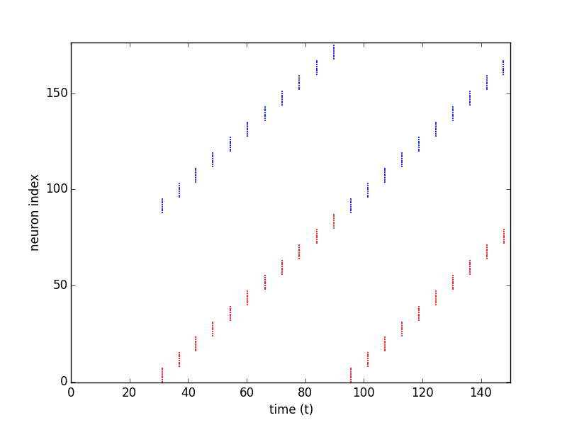
We present here a simple example network, a toy model of a “synfire chain”, in which the activity propagates across the network.

As with any Python script, the first step is to import the external libraries that we will use. Here we import the NEST backend of PyNN for the simulation, NumPy for random number generation, and matplotlib for plotting.

import pyNN.nest as sim
import numpy.random
import matplotlib.pyplot as plt

Next we define numerical parameters, such as the number and size of neuronal populations, neuron properties, synaptic weights and delays, etc.

n_populations = 11
population_size = 8
neuron_parameters = {
    'cm': 0.2,
    'v_reset': -70,
    'v_rest': -70,
    'v_thresh': -47,
    'e_rev_I': -70,
    'e_rev_E': 0.0,
}
weight_exc_exc = 0.005
weight_exc_inh = 0.005
weight_inh_exc = 0.5
delay = 3.0
rng_seed = 42
stimulus_onset = 25.0
stimulus_sigma = 0.5
runtime = 150.0

The setup() function initializes and configures the simulator (in this case NEST).

sim.setup(timestep=0.1)

The main building block in PyNN is a population of neurons of the same type (although the parameters of the neurons within the population can be heterogeneous). Here we create 11 populations of excitatory integrate-and-fire (IF) neurons and 11 populations of inhibitory IF neurons.

populations = {'exc': [], 'inh': []}
for syn_type in ('exc', 'inh'):
    populations[syn_type] = [sim.Population(population_size,
                                            sim.IF_cond_exp,
                                            neuron_parameters)
                             for i in range(n_populations)]

We now connect each excitatory population to the following pair of excitatory and inhibitory populations, and each inhibitory population to the excitatory population within the same pair.

connector_exc_exc = sim.AllToAllConnector(weights=weight_exc_exc, delays=delay)
connector_exc_inh = sim.AllToAllConnector(weights=weight_exc_inh, delays=delay)
connector_inh_exc = sim.AllToAllConnector(weights=weight_inh_exc, delays=delay)

for i in range(n_populations):
    j = (i + 1) % n_populations
    prj_exc_exc = sim.Projection(populations['exc'][i], populations['exc'][j],
                                 connector_exc_exc, target='excitatory')
    prj_exc_inh = sim.Projection(populations['exc'][i], populations['inh'][j],
                                 connector_exc_inh, target='excitatory')
    prj_inh_exc = sim.Projection(populations['inh'][i], populations['exc'][i],
                                 connector_exc_exc, target='inhibitory')

The first pair of populations are stimulated by a burst of spikes.

numpy.random.seed(rng_seed)
stim_spikes = numpy.random.normal(loc=stimulus_onset,
                                  scale=stimulus_sigma,
                                  size=population_size)
stim_spikes.sort()
stimulus = sim.Population(1, sim.SpikeSourceArray, {'spike_times': stim_spikes})

prj_stim_exc = sim.Projection(stimulus, populations['exc'][0],
                              connector_exc_exc, target='excitatory')
prj_stim_inh = sim.Projection(stimulus, populations['inh'][0],
                              connector_exc_inh, target='excitatory')

We’ve now finished building the network, now we instrument it, by recording spikes from all populations.

for syn_type in ('exc', 'inh'):
    for population in populations[syn_type]:
        population.record()

Now we run the simulation:

sim.run(runtime)

Finally we loop over the populations, retrieve the spike times, and plot a raster plot (spike time vs neuron index).

colours = {'exc': 'r', 'inh': 'b'}

id_offset = 0
for syn_type in ['exc', 'inh']:
    for population in populations[syn_type]:
        spikes = population.getSpikes()
        colour = colours[syn_type]
        plt.plot(spikes[:,1], spikes[:,0] + id_offset,
                 ls='', marker='o', ms=1, c=colour, mec=colour)
        id_offset += population.size

plt.xlim((0, runtime))
plt.ylim((-0.5, 2* n_populations * population_size + 0.5))
plt.xlabel('time (t)')
plt.ylabel('neuron index')
plt.savefig("synfire_chain.png")

Note that here we include the plotting in the same script to illustrate the example output. Scripts submitted to the Neuromorphic Computing Platform can also save spikes to file and use the other tools available in the EBRAINS research infrasstructure for analysing and visualizing the results.

Using different backends¶

To run the same simulation with a different simulator, just change the name of the PyNN backend to import, e.g.:

import pyNN.neuron as sim

to run the simulation with NEURON. For the PM system, the module to import is pyNN.hardware.hbp_pm while for the MC system the module is pyNN.spiNNaker.

The recommended approach is to provide the name of the backend as a command-line argument, i.e., you run your simulation using:

$ python run.py nest

PyNN contains some utility functions to make this easier. With PyNN 0.7, use:

from pyNN.utility import get_script_args
simulator_name = get_script_args(1)[0]
exec("import pyNN.%s as sim" % simulator_name)

With PyNN 0.8:

from pyNN.utility import get_simulator
sim, options = get_simulator()

“Physical model” (BrainScaleS) system¶

The BrainScaleS system has a number of additional configuration options that can be passed to setup(). These are explained in About the BrainScaleS hardware. There are also a number of limitations, for example only a subset of the PyNN standard neuron and synapse models are available.

The BrainScaleS system attempts to automatically place neurons on the wafers in an optimal way. However, it is possible to influence this placement or control it manually. An example can be found in label-marocco-example.

“Many core” (SpiNNaker) system¶

The SpiNNaker system supports the standard arguments provided by the PyNN setup() function. The SpiNNaker system has a number of limitations in terms of the support for PyNN functionality, for example, only a subset of the PyNN standard neuron and synapse models are currently available. These limitations are defined in the online documentation here.

The SpiNNaker software stack attempts to automatically partition the populations defined in the PyNN script into core sized chunks (the smallest atomic size of resource for a machine) of neurons which are then placed onto the machine in an optimal way in regard to the machine’s available resources. However, it is possible to influence the partitioning and placement behaviours manually.

For example, take the PyNN definition of a population from the “synfire chain” example discussed previously, and shown below:

populations[syn_type] = sim.Population(population_size,
                                       sim.IF_cond_exp,
                                       neuron_parameters)

A constraint can be added to the model which can limit how many neurons each core will contain at a maximum. This is shown below:

populations[syn_type] = sim.Population(population_size,
                                       sim.IF_cond_exp,
                                       neuron_parameters)
sim.set_number of_neurons_per_core(sim.IF_cond_exp, 200)

This and other examples of manual limitations can be found in the online documentation here.