BrainScaleS-2 single neuron experiments

In order to use the microscheduler we have to set some environment variables first:

from _static.common.helpers import setup_hardware_client
setup_hardware_client()

%matplotlib inline
import numpy as np
from ipywidgets import interact, IntSlider
from functools import partial
IntSlider = partial(IntSlider, continuous_update=False)
import matplotlib.pyplot as plt
plt.style.use("_static/matplotlibrc")

import pynn_brainscales.brainscales2 as pynn
from pynn_brainscales.brainscales2 import Population
from pynn_brainscales.brainscales2.standardmodels.cells import SpikeSourceArray
from pynn_brainscales.brainscales2.standardmodels.synapses import StaticSynapse


def plot_membrane_dynamics(population: Population, segment_id=-1, ylim=None):
    """
    Plot the membrane potential of the neuron in a given population view. Only
    population views of size 1 are supported.
    :param population: Population, membrane traces and spikes are plotted for.
    :param segment_id: Index of the neo segment to be plotted. Defaults to
                       -1, encoding the last recorded segment.
    :param ylim: y-axis limits for the plot.
    """
    if len(population) != 1:
        raise ValueError("Plotting is supported for populations of size 1.")
    # Experimental results are given in the 'neo' data format
    mem_v = population.get_data("v").segments[segment_id].irregularlysampledsignals[0]

    plt.plot(mem_v.times, mem_v, alpha=0.5)
    print(f"Mean membrane potential: {mem_v.mean()}")
    plt.xlabel("Wall clock time [ms]")
    plt.ylabel("ADC readout [a.u.]")
    if ylim:
        plt.ylim(ylim)

In this part we will explore some of the spiking capabilities of the BrainScaleS-2 neuromorphic accelerator using our implementation of the pyNN interface.

There are 512 neuron compartments emulating the leaky integrate and fire model and 131,072 STP/STDP synapses in one HICANN-X chip, but we will stick to a single neuron for now.

A silent neuron

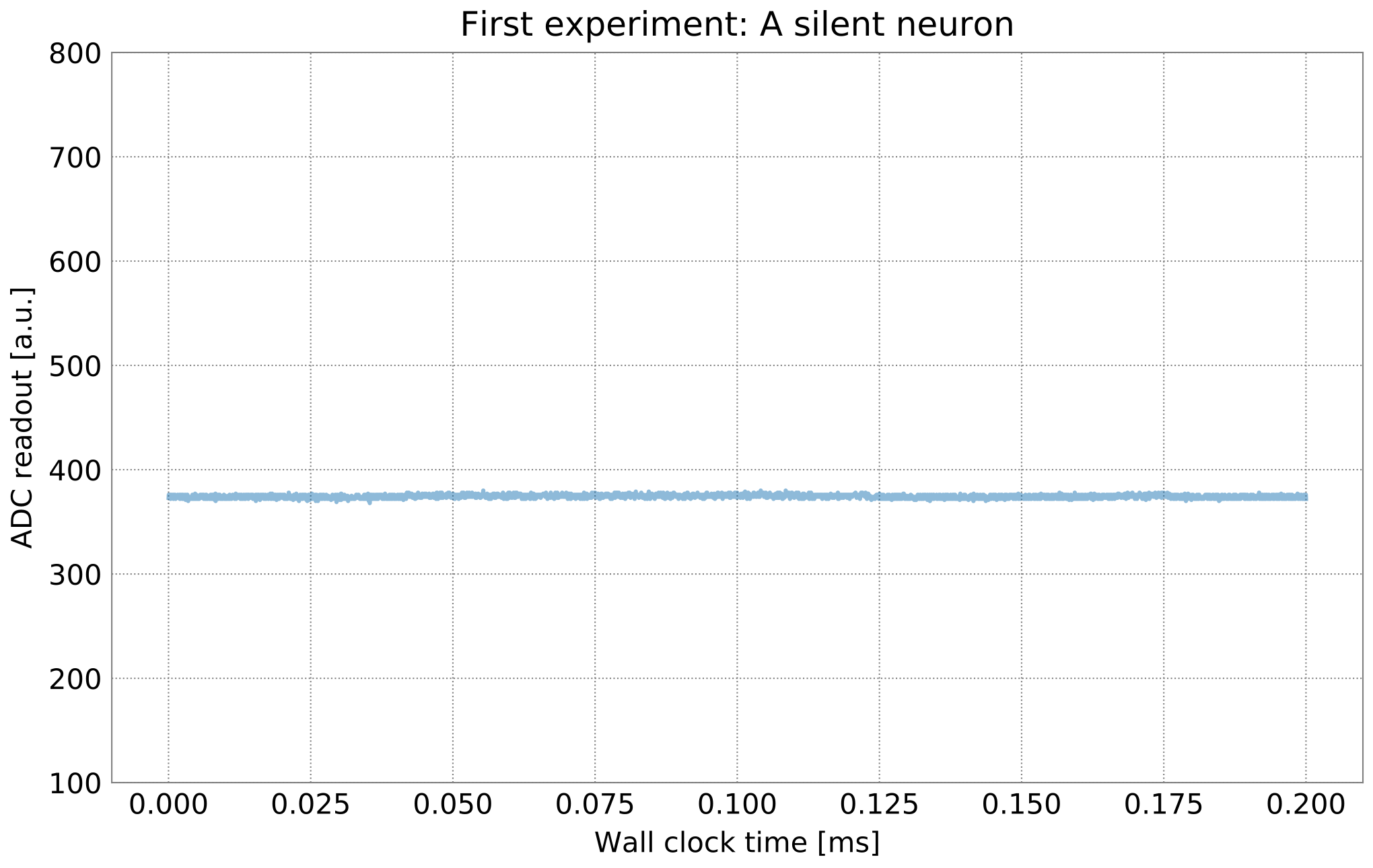
As a first experiment, we will record the membrane of a single, silent neuron on the analog substrate. We use pyNN as an interface, which can be used similarly to existing simulators and other neuromorphic platforms.

While we provide calibrated neurons that have their hardware parameters set to match high-level targets, e.g., time-constants, we will start with modifying a few circuit parameters directly. These control the dynamic behavior of the neuron as well as static configuration. Most of them are either boolean or given in units of ‘LSB’ for chip-internal Digital-to-Analog converters, providing voltages and currents - they have no direct biological translation.

For this first example, you may alter the leak potential via the slider and observe the response of the analog neuron’s resting potential.

We first define a population of one neuron and let its membrane potential be recorded. The experiment is executed by calling pynn.run(time_in_ms). The network is evolved for a given amount of time and neurons are stimulated by any given stimuli.

The time is given in units of milliseconds (wall clock time), representing the hardware’s intrinsic 1000-fold speed-up compared to biological systems.

@interact(v_leak=IntSlider(min=400, max=1022, step=1, value=700))
def experiment(v_leak):
    plt.figure()
    plt.title("First experiment: A silent neuron")

    pynn.setup()

    pop = pynn.Population(1, pynn.cells.HXNeuron(
        # Leak potential, range: 400-1000
        leak_v_leak=v_leak,
        # Leak conductance, range: 0-1022
        leak_i_bias=1022))

    # The chip contains a fast Analog-to-Digital converter. It can be used to
    # record different observables of a single analog neuron - most importantly
    # the membrane potential.
    pop.record(["v"])

    # Execute experiment
    pynn.run(0.2)

    plot_membrane_dynamics(pop, ylim=(100, 800))
    plt.show()

    # Reset the pyNN internal state and prepare for the following experiment.
    pynn.end()

Leak over threshold

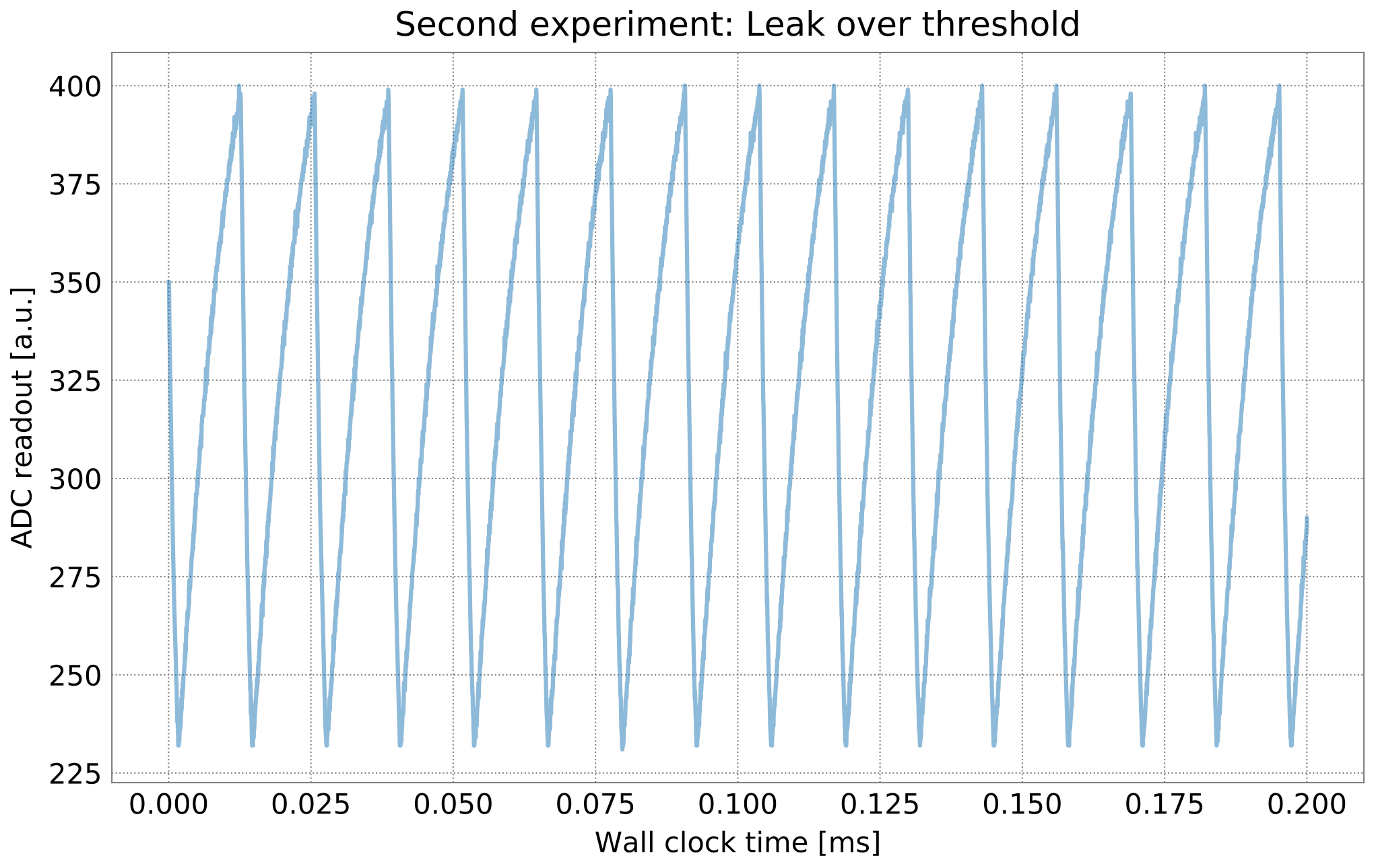
As a second experiment, we will let the neurons on BrainScaleS-2 spike by setting a ‘leak-over-threshold’ configuration. The leak potential is set high, above the spike threshold, so that the membrane charges exponentially until a spike is triggered. The potential is then reset to a lower voltage.

The parametrization of the different potentials is not equal, a lower threshold setting of 300 may correspond to a higher leak potential of 700.

@interact(
    v_leak=IntSlider(min=400, max=1022, step=1, value=1000),
    v_threshold=IntSlider(min=0, max=500, step=1, value=300),
    v_reset=IntSlider(min=300, max=1022, step=1, value=400),
    i_bias_leak=IntSlider(min=0, max=1022, step=1, value=150),
)
def experiment(v_leak, v_threshold, v_reset, i_bias_leak):
    """
    Set up a leak over threshold neuron.

    :param v_leak: Leak potential.
    :param v_threshold: Spike threshold potential.
    :param v_reset: Reset potential.
    :param i_bias_leak: Controls the leak conductance (membrane time constant).
    """

    plt.figure()
    plt.title("Second experiment: Leak over threshold")

    pynn.setup()

    pop = pynn.Population(1, pynn.cells.HXNeuron(
        # Leak potential, range: 400-1000
        leak_v_leak=v_leak,
        # Leak conductance, range: 0-1022
        leak_i_bias=i_bias_leak,
        # Threshold potential, range: 0-500
        threshold_v_threshold=v_threshold,
        # Reset potential, range: 300-1000
        reset_v_reset=v_reset,
        # Membrane capacitance, range: 0-63
        membrane_capacitance_capacitance=63,
        # Refractory time (counter), range: 0-255
        refractory_period_refractory_time=255,
        # Enable reset on threshold crossing
        threshold_enable=True,
        # Reset conductance, range: 0-1022
        reset_i_bias=1022,
        # Increase reset conductance
        reset_enable_multiplication=True))

    pop.record(["v", "spikes"])
    pynn.run(0.2)
    plot_membrane_dynamics(pop, ylim=(100, 800))
    plt.show()
    pynn.end()

The neuron has many more parameters you may play around with. Some documentation for these parameters is available in our Lower-level API documentation. The kewords you set in PyNN are generated from a hierarchical structure – search for the last part of a parameter (e.g. capacitance).

pynn.cells.HXNeuron().get_parameter_names()

Fixed-pattern variations

Due to the analog nature of the BrainScaleS-2 platform, the inevitable mismatch of semiconductor fabrication results in inhomogeneous properties of the computational elements.

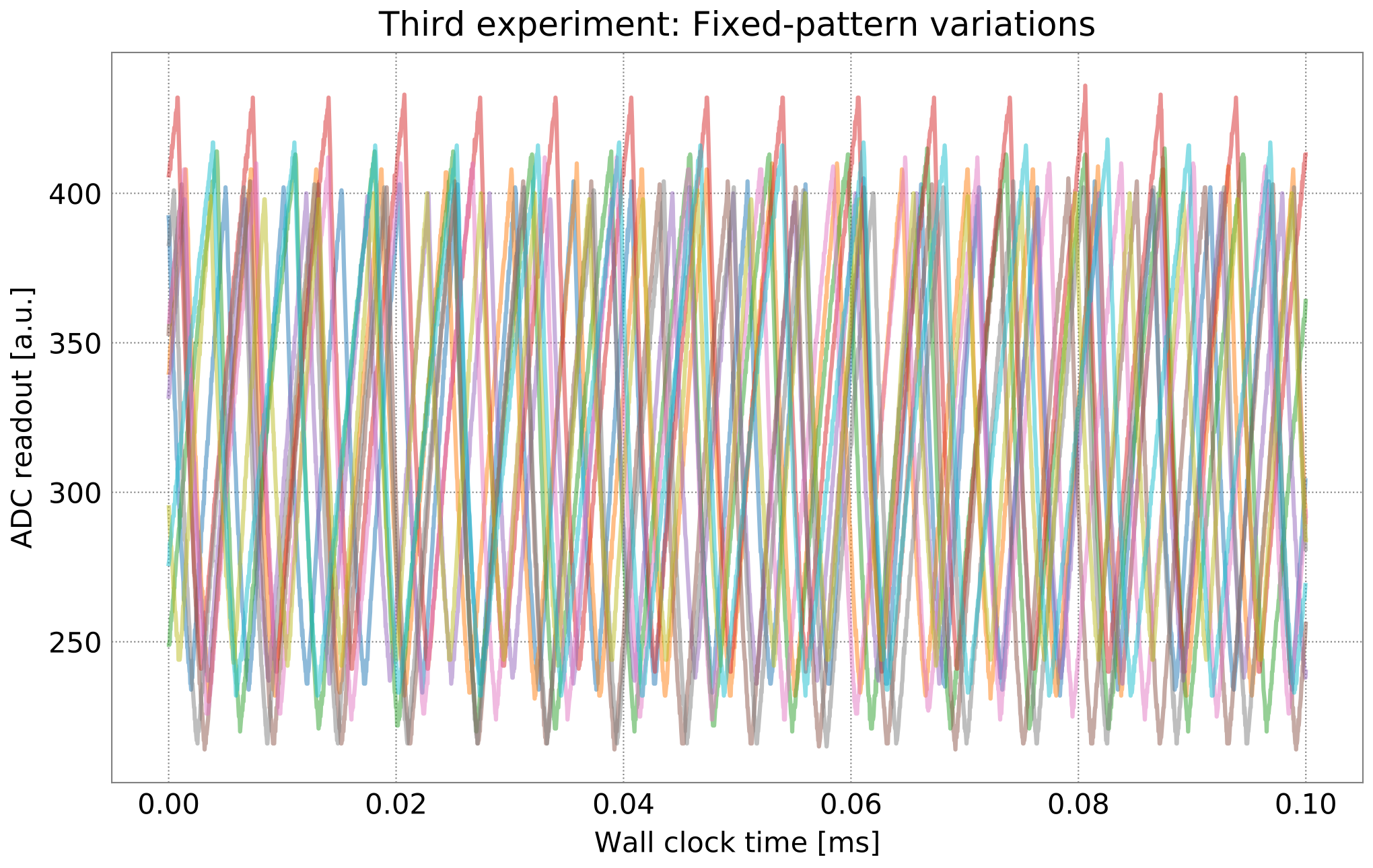
We will visualize these effects by recording the membrane potential of multiple neurons in leak-over-threshold configuration. You will notice different resting, reset and threshold potentials as well as varying membrane time constants.

plt.figure()
plt.title("Third experiment: Fixed-pattern variations")

pynn.setup()

pop = pynn.Population(10, pynn.cells.HXNeuron(
    # Leak potential, range: 400-1000
    leak_v_leak=1000,
    # Leak conductance, range: 0-1022
    leak_i_bias=200,
    # Threshold potential, range: 0-600
    threshold_v_threshold=500,
    # Reset potential, range: 300-1000
    reset_v_reset=400,
    # Membrane capacitance, range: 0-63
    membrane_capacitance_capacitance=63,
    # Refractory time, range: 0-255
    refractory_period_refractory_time=255,
    # Enable reset on threshold crossing
    threshold_enable=True,
    # Reset conductance, range: 0-1022
    reset_i_bias=1022,
    # Increase reset conductance
    reset_enable_multiplication=True))

for neuron_id in range(len(pop)):
    print(f"Recording fixed-pattern variations: Run {neuron_id}")
    p_view = pynn.PopulationView(pop, [neuron_id])
    p_view.record(["v"])
    pynn.run(0.1)
    plot_membrane_dynamics(p_view, ylim=(100, 800))
    pynn.reset()
    pop.record(None)

plt.show()
pynn.end()

The plot shows the recorded membrane traces of multiple different neurons. Due to the time-continuous nature of the system, there is no temporal alignment between the individual traces, so the figure shows multiple independent effects:

• Temporal misalignment: From the system’s view, the recording happens in an arbitrary time frame during the continuously evolving integration. Neurons are not synchronized to each other.

• Circuit-level mismatch: Each individual neurons shows slightly different analog properties. The threshold is different for all traces; as is the membrane time constant (visible as slope) and the reset potentials (visible as plateaus during the refractory time).

Summary

The analog neurons on BrainScaleS-2 feature many hardware parameters that can be set to achieve different operating points and to equalize the behaviour of different neurons.

We will employ an automated calibration to get the neurons in the desired operating mode. * In the next notebook, we will show spiking operation and learning. * Later, we will change the target parameters and use integrator neurons for executing multiply-accumulate operations.

Outlook: External stimulation

We will continue the tutorial in the next notebook using external stimulation on the neurons. You may play around a bit already here, but we will revisit the following later.

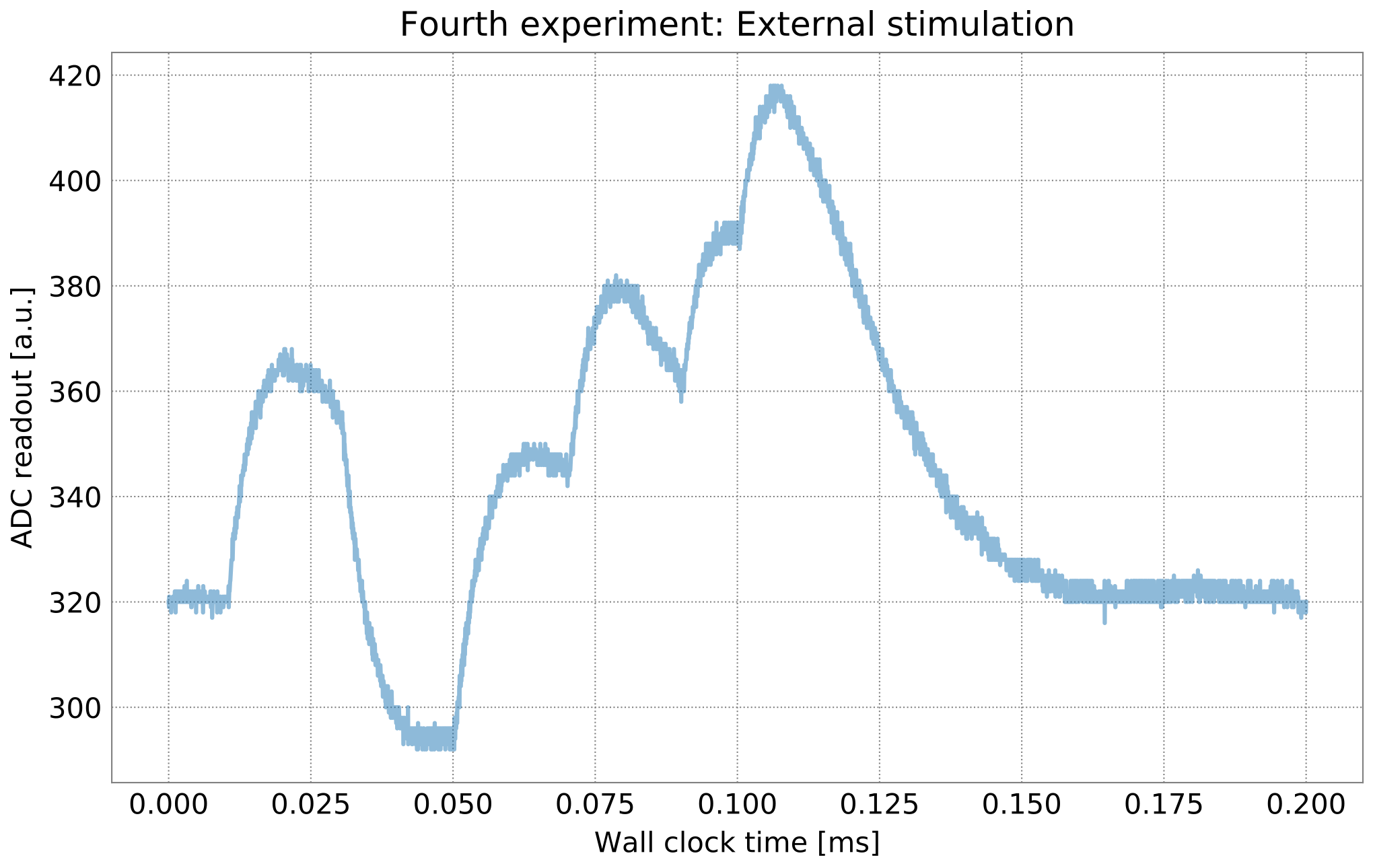
Up to now, we have observed analog neurons without external stimulus. In this experiment, we will introduce the latter and examine post-synaptic pulses on the analog neuron’s membrane.

Preparing the neuron to receive synaptic inputs requires the configuration of additional circuits. The additional settings include technical parameters for bringing the circuit to its designed operating point as well as configuration with a direct biological equivalent. For simplicity, we will turn to a calibration which yields all required parameters and counters the fixed pattern noise between different neurons observed previously.

We represent projections as entries in the synapse matrix on the neuromorphic chip. Weights are stored in digital 6bit values (plus sign), the value range for on-chip weights is therefore -63 to 63. With this first projection, we connect the external spike source to the observed on-chip neuron population.

A default calibration is generated for every setup every night. We save the nightly calibration in two variables such that we can use it later when we define our neuronal network.

from _static.common.helpers import get_nightly_calibration
calib = get_nightly_calibration()

Now we can continue by defining our experiment:

@interact(exc_weight=IntSlider(min=0, max=63, step=1, value=31),
          inh_weight=IntSlider(min=0, max=63, step=1, value=31),
          isi=IntSlider(min=10, max=100, step=5, value=50))
def run_experiment(exc_weight: int, inh_weight: int, isi: float):
    '''
    Run external input demonstration on BSS-2.

    Adjust weight of projections, set input spikes and execute experiment
    on BSS-2.

    :param exc_weight: Weight of excitatory synaptic inputs, value range
        [0,63].
    :param inh_weight: Weight of inhibitory synaptic inputs, value range
        [0,63].
    :param isi: Time between synaptic inputs in microsecond (hardware
        domain)
    '''

    plt.figure()
    plt.title("Fourth experiment: External stimulation")

    pynn.setup(initial_config=calib)

    # use calibrated parameters for neuron
    stimulated_p = pynn.Population(1, pynn.cells.HXNeuron())
    stimulated_p.record(["v", "spikes"])

    # calculate spike times
    wait_before_experiment = 0.01  # ms (hw)
    isi_ms = isi / 1000  # convert to ms
    spiketimes = np.arange(6) * isi_ms + wait_before_experiment

    # all but one input are chosen to be exciatory
    excitatory_spike = np.ones_like(spiketimes, dtype=bool)
    excitatory_spike[1] = False

    # external input
    exc_spikes = spiketimes[excitatory_spike]
    exc_stim_pop = pynn.Population(2, SpikeSourceArray(spike_times=exc_spikes))
    exc_proj = pynn.Projection(exc_stim_pop, stimulated_p,
                               pynn.AllToAllConnector(),
                               synapse_type=StaticSynapse(weight=exc_weight),
                               receptor_type="excitatory")

    inh_spikes = spiketimes[~excitatory_spike]
    inh_stim_pop = pynn.Population(2, SpikeSourceArray(spike_times=inh_spikes))
    inh_proj = pynn.Projection(inh_stim_pop, stimulated_p,
                               pynn.AllToAllConnector(),
                               synapse_type=StaticSynapse(weight=-inh_weight),
                               receptor_type="inhibitory")

    # run experiment
    pynn.run(0.6)
    plot_membrane_dynamics(stimulated_p, ylim=(100, 600))
    plt.show()
    pynn.end()

You may play around with the parameters in this experiment to achieve different traces. Try to stack multiple PSPs, try to make the neuron spike more often, be creative!