Learning with the SuperSpike rule
In the previous example, you accustomed yourself with BrainScaleS-2’s analog neuron circuit. Here, we will build on this knowledge and train a single neuron to reproduce a pre-defined target spike train. For this purpose, we will implement the SuperSpike learning rule [1] to minimize the van Rossum distance between the targets and the spikes produced by our neuron.
Specifically, we will
set up a network using PyNN,
generate a target spike train,
re-initialize the network’s weights,
and implement an in-the-loop training scheme directly in Python.
Training spiking networks with surrogate gradients
The discontinuity introduced by the spiking threshold presents challenges when it comes to training networks of spiking neurons with gradient-based methods, especially when employing sparse coding techniques far away from the rate coding limit. Recently, efforts have been made by “smoothing” out the true activation function for the backward pass [1,2,3,4,5]. These “surrogate gradients” allow to easily train feed-forward as well as recurrent SNNs on common benchmark datasets.
For BrainScaleS-2, we have developed a powerful in-the-loop training scheme that allows to perform backpropagation through time using auto-differentiation frameworks [6]. With a feed-forward network, we reached 97.6 % test accuracy on the MNIST dataset. The accelerated emulation allowed to classify more than 85k images per second with an energy budget of only 2.4 μJ per image. Moreover, we trained a recurrent SNN on natural language data from the SHD dataset [7].
In this example, we will not go that far. Instead, we will implement the forward-integrated SuperSpike learning rule on a simple artifical input pattern. In case you are interested, though, please refer to the original publication.
References for further reading
Zenke, Friedemann, and Surya Ganguli. “Superspike: Supervised learning in multilayer spiking neural networks.” Neural computation 30.6 (2018): 1514-1541.
Neftci, Emre O., Hesham Mostafa, and Friedemann Zenke. “Surrogate gradient learning in spiking neural networks: Bringing the power of gradient-based optimization to spiking neural networks.” IEEE Signal Processing Magazine 36.6 (2019): 51-63.
Bellec, Guillaume, et al. “A solution to the learning dilemma for recurrent networks of spiking neurons.” Nature communications 11.1 (2020): 1-15.
Bohte, Sander M. “Error-backpropagation in networks of fractionally predictive spiking neurons.” International Conference on Artificial Neural Networks. Springer, Berlin, Heidelberg, 2011.
Esser, Steven K., et al. “Convolutional networks for fast, energy-efficient neuromorphic computing.” Proceedings of the national academy of sciences 113.41 (2016): 11441-11446.
Cramer, Benjamin, et al. “Surrogate gradients for analog neuromorphic computing” Proceedings of the national academy of sciences 119.4 (2022)
Cramer, Benjamin, et al. “The Heidelberg Spiking Data Sets for the Systematic Evaluation of Spiking Neural Networks.” IEEE Transactions on Neural Networks and Learning Systems (2020).
In order to use the microscheduler we have to set some environment variables first:
from _static.common.helpers import setup_hardware_client
setup_hardware_client()
%matplotlib inline
import numpy as np
import ipywidgets as w
import matplotlib.pyplot as plt
from contextlib import suppress
with suppress(IOError):
    plt.style.use("_static/matplotlibrc")

import pynn_brainscales.brainscales2 as pynn
np.random.seed(1234)
Helper functions
Let’s define some helper functions for plotting.
def create_figure():
    fig, axes = plt.subplots(2, 1)

    axes[0].set_ylabel("norm. membrane")
    axes[0].set_xlim(0, duration * 1e6)
    axes[0].set_xticklabels([])
    axes[0].plot([], [], c="C0")
    axes[0].set_ylim(-0.1, 1.1)

    axes[1].set_xlabel("time / μs")
    axes[1].set_ylabel("error trace")
    axes[1].set_xlim(0, duration * 1e6)
    axes[1].plot([], [], c="C0")
    axes[1].set_ylim(-0.5, 0.5)

    return fig, axes

def update_figure(fig, *data):
    for ax, d in zip(fig.axes, data):
        ax.get_lines()[0].set_data(d[0] * 1e6, d[1])
    display(fig)
Define network in PyNN
First, we will set up some variables determining the network structure. We will furthermore define the binning of the stimuli and the later calculation of the weight updates.
n_inputs = 25

duration = 200e-6  # s in wallclock time
dt = 0.1e-6

n_steps = int(duration / dt)

time = np.arange(n_steps) * dt
bins = np.arange(n_steps + 1) * dt
Before we define our network, we load the default calibration.
A default calibration is generated for every setup every night. We save the nightly calibration in a variable such that we can use it later when we define our experiment.
from _static.common.helpers import get_nightly_calibration
calib = get_nightly_calibration()
Now, we can define the network itself using PyNN.
# setup PyNN and inect calibration data
pynn.setup(initial_config=calib)

# create output population (one neuron) and record its observables
pop_output = pynn.Population(1, pynn.cells.HXNeuron())
pop_output.record(["spikes", "v"])

# create spike sources
pop_input = pynn.Population(n_inputs, pynn.cells.SpikeSourceArray(spike_times=[]))

# define two projections (excitatory + inhibitory) to allow signed weights
synapse_exc = pynn.standardmodels.synapses.StaticSynapse(weight=42)
synapse_inh = pynn.standardmodels.synapses.StaticSynapse(weight=-42)
projection_io_inh = pynn.Projection(pop_input, pop_output,
                             pynn.AllToAllConnector(),
                             synapse_type=synapse_inh,
                             receptor_type="inhibitory")
projection_io_exc = pynn.Projection(pop_input, pop_output,
                             pynn.AllToAllConnector(),
                             synapse_type=synapse_exc,
                             receptor_type="excitatory")
To work around Dale’s law, we have to merge two projections together to form signed synapses. The following function assigns the signed weight matrix to the two projections.
def set_weights(weights, w_max=63):
    # limit weights to hw boundaries
    weights = weights.clip(-w_max, w_max)

    integer_weights = np.round(weights).astype(int)
    w_exc = integer_weights * (integer_weights >= 0).astype(int)
    w_inh = integer_weights * (integer_weights < 0).astype(int)

    projection_io_inh.set(weight=w_inh)
    projection_io_exc.set(weight=w_exc)
Construct Poisson input spike trains
To generate (fixed-seed) random inputs, we calculate binned spike trains according to a Bernoulli process.
np.random.seed(123456)

freq = 10e3  # Hz (remember the acceleration factor!)
input_spikes = []
stimuli_dense = np.random.rand(n_inputs, n_steps) < freq * dt
stimuli_dense[:, (time > (duration - 20e-6))] = 0

for s in stimuli_dense:
    input_spikes.append(np.where(s)[0] * dt * 1e3) # convert to ms for pyNN

pop_input.set(spike_times=input_spikes)
Generating a taget spike train
Now, we can inject the previously defined input spike trains into our target neuron. For this purpose, we first randomly initialize the synaptic weights.
The resulting output spikes will later be used as a target spike train. The difficulty of the task will depend on the number and timing of target spikes.
Exercises
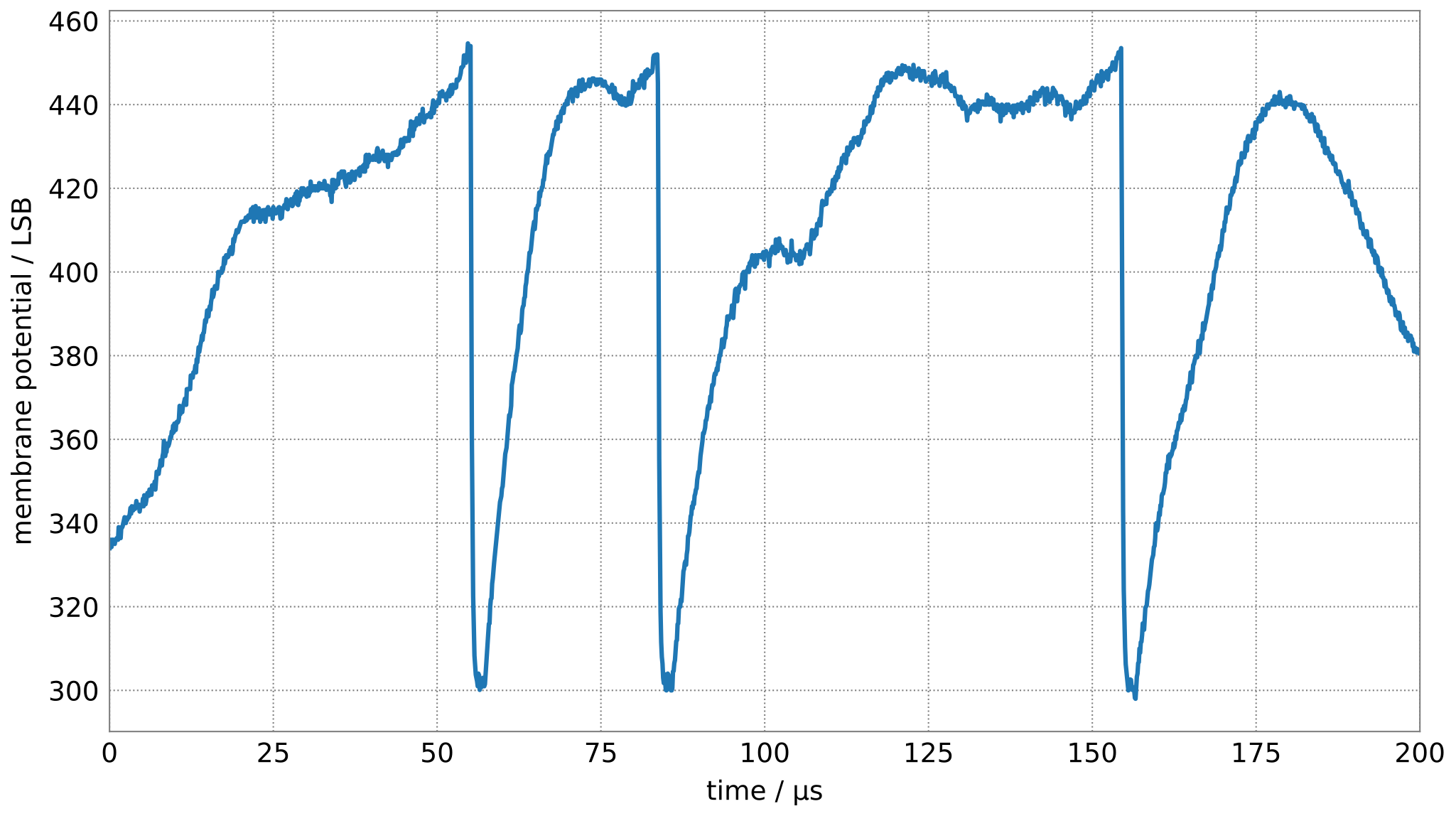
Play around with the mean and standard deviation of the weight distribution and observe the output of the neuron. Try to get the neuron to emit approximately 3 to 4 spikes. This spike train will later be used as a target spike train \(\hat S_i\).
@w.interact(
    weight_mean=w.FloatSlider(
        27, min=0, max=40, continuous_update=False),
    weight_std=w.FloatSlider(
        1, min=0, max=10, continuous_update=False)
)
def experiment(weight_mean, weight_std):
    global v_mem, target_spikes
    np.random.seed(123)
    weights = np.random.normal(weight_mean, weight_std, size=(n_inputs, 1))
    set_weights(weights)
    pynn.run(duration * 1e3)

    data = pop_output.get_data()

    target_spikes = data.segments[-1].spiketrains[0] / 1e3  # convert ms to s

    membrane = data.segments[-1].irregularlysampledsignals[0]
    v_mem = np.interp(time, membrane.times / 1e3, membrane.magnitude[:, 0])

    fig = plt.figure()
    ax = fig.gca()
    ax.plot(time*1e6, v_mem)

    ax.set_xlim(0, duration*1e6)
    ax.set_xlabel("time / μs")
    ax.set_ylabel("membrane potential / LSB")
    pynn.reset()
experiment(27, 1); plt.close()  # needed for testing

Extract the dynamic range from the above plot to normalize the membrane potential for calculating the surrogate gradient.
v_zero = v_mem.min()
dynamic_range = v_mem.max() - v_zero
The SuperSpike learning rule
The SuperSpike learning rule was derived to perform gradient descent on the van Rossum distance
between the current spike train \(S_i\) and the target spike train \(\hat S_i\). Here, \(\alpha\) is the kernel used to calculate the van Rossum distance and \(e_i(s)\) the error signal. The weight update rule can in the end be written as
where \(\sigma^\prime\) represents the surrogate gradient of membrane potential \(v_i\), and \(\epsilon\) the exponentially decaying kernel of the synaptic currents.
The integral consists of a Hebbian contribution which combines the surrogate gradient of the membrane potential with the exponentially decaying synaptic currents as eligibility traces. This term is augmented by the error signal as a third factor, which can be calculated through backpropagation for multi-layer networks.
The learning rule can be forward-integrated alongside the neuronal dynamics, which makes it particularly interesting for online learning applications.
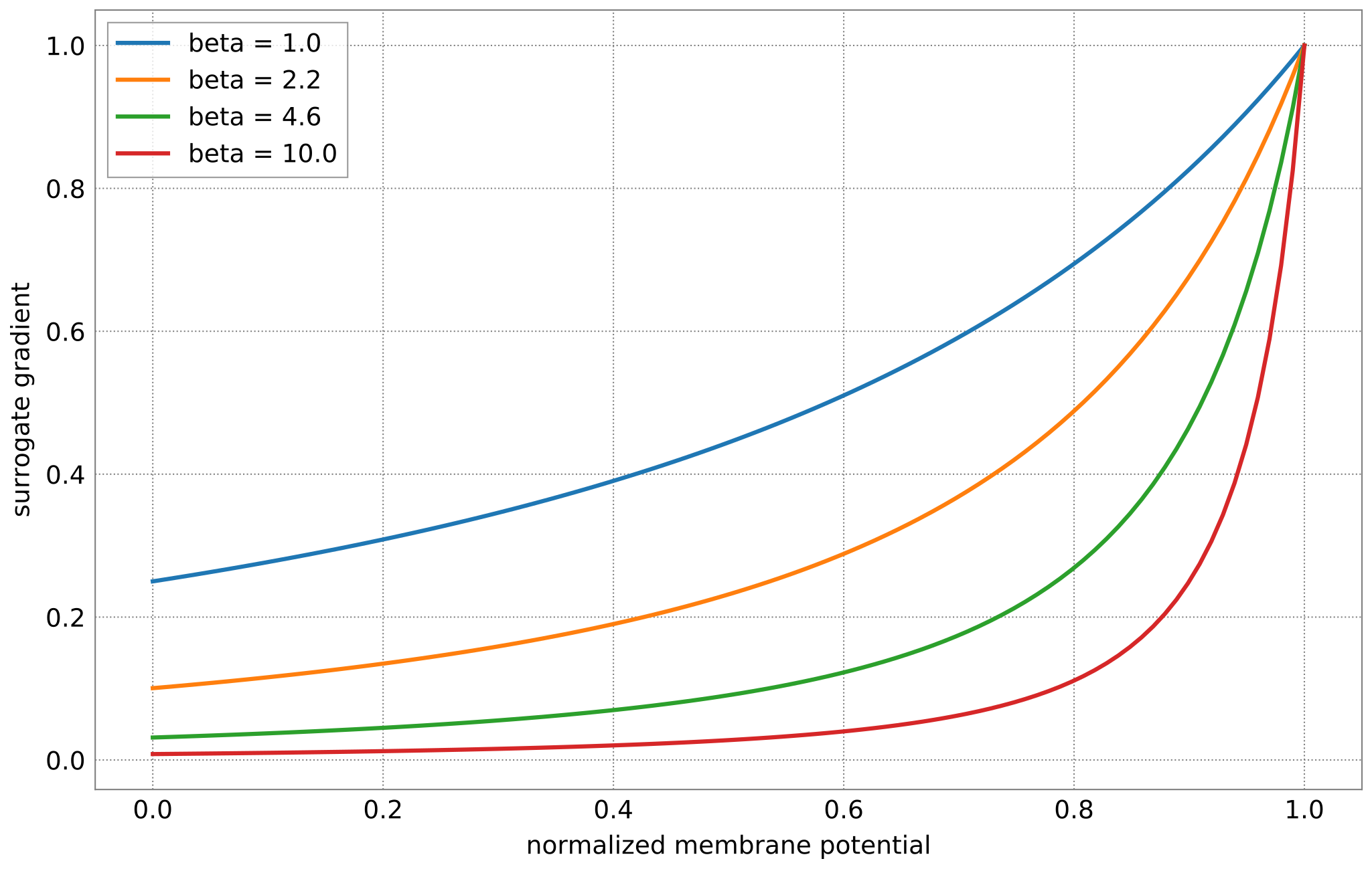
Let’s have a look at the surrogate function \(\sigma^\prime\) as a function of the steepness paramter \(\beta\).
def superspike(v_m, beta=5.0):
    return np.power(1 + np.abs(beta * (v_m - 1.0)), -2)

fig = plt.figure()
ax = fig.gca()

v = np.linspace(0, 1, 100)

for beta in np.logspace(np.log10(1), np.log10(10), 4):
    ax.plot(v, superspike(v, beta=beta), label=f"beta = {beta:.1f}")

ax.legend(loc="upper left")
ax.set_xlabel("normalized membrane potential")
ax.set_ylabel("surrogate gradient");

The SuperSpike learning rules requires estimates of the neuro-synaptic time constants. Here, we use the same values as targeted for the deployed calibration data.
tau_mem = 10e-6
tau_syn = 5e-6
Construct kernels for the learning rule, including the van Rossum distance.
n_kernel_steps = int(100e-6 / dt)
n_kernel_steps = n_kernel_steps + (1 - n_kernel_steps % 2)

kernel_psc = np.zeros(n_kernel_steps)
kernel_psc[-int(kernel_psc.size / 2):] += np.exp(-np.arange(int(kernel_psc.size / 2)) / (tau_syn / dt))

kernel_psp = kernel_psc.copy()
kernel_psp[-int(kernel_psp.size / 2):] -= np.exp(-np.arange(int(kernel_psp.size / 2)) / (tau_mem / dt))

kernel_vrd = kernel_psp.copy()
Training the network
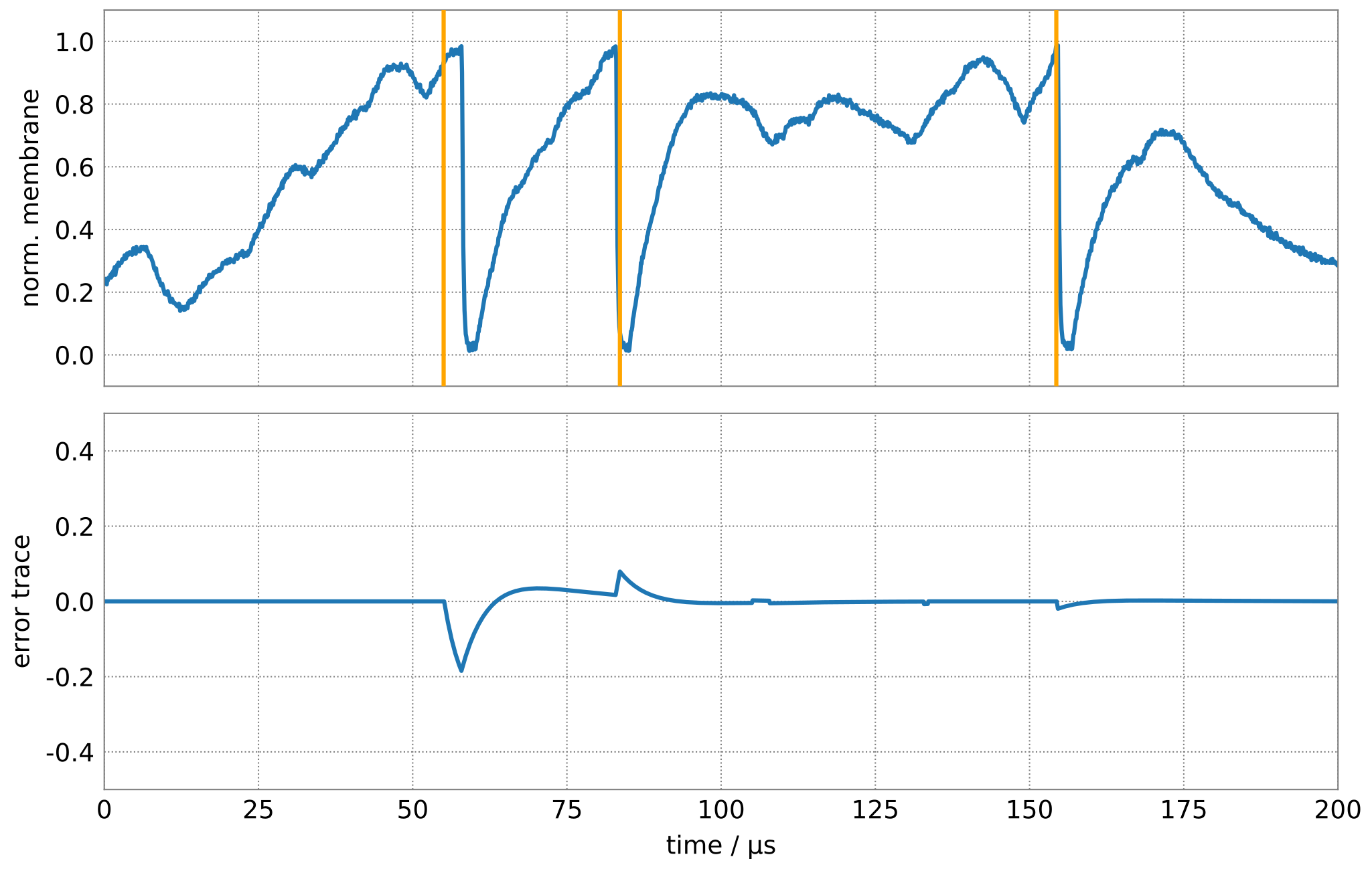
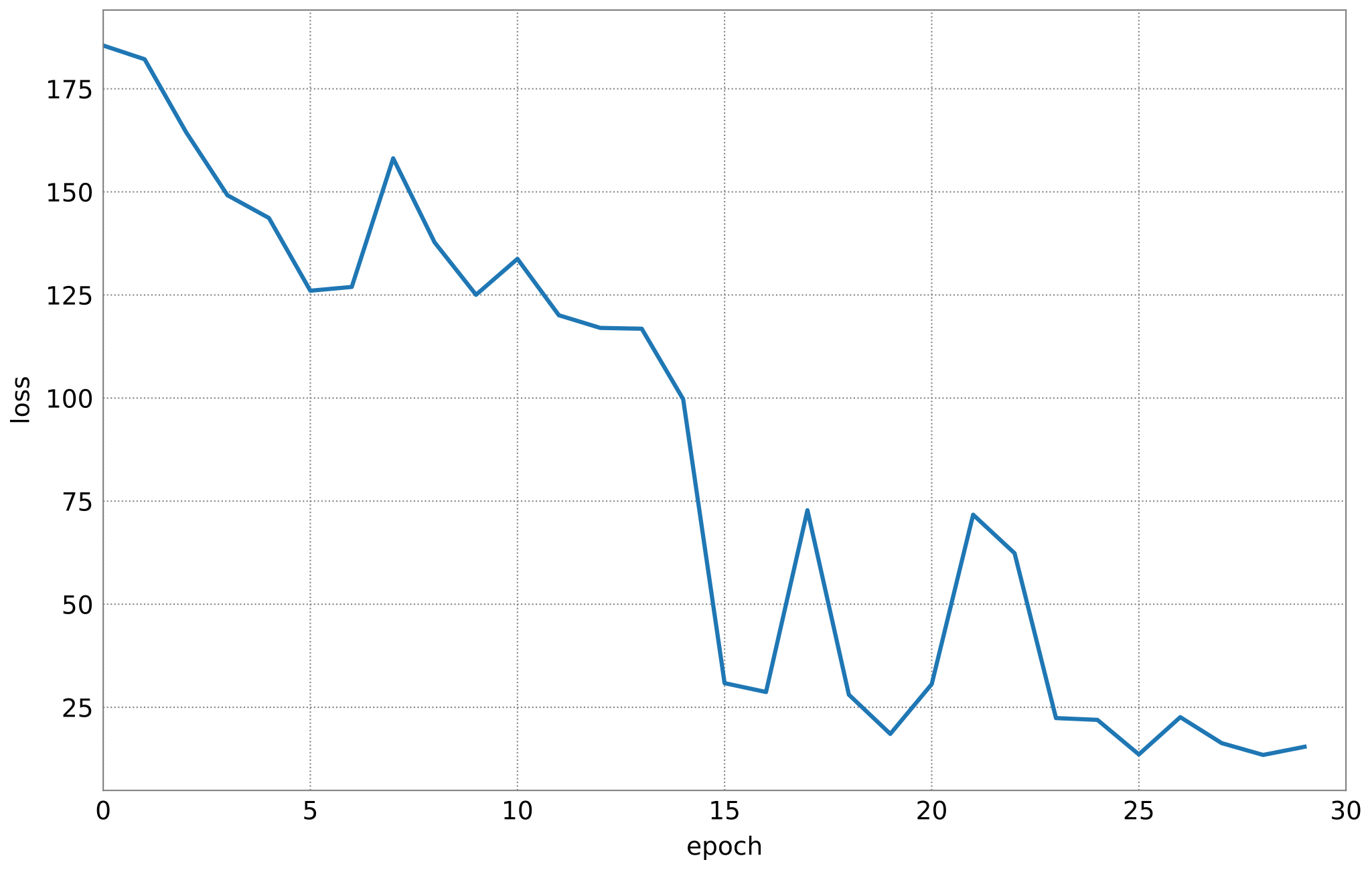
We can now implement above’s weight update expression in Python and use it to train our network to replicate the target spike train generated above.
Exercises
Train the network for different target spike trains (\(\hat S_i\)). For that purpose, modify above’s cell for the target generation (e.g. seed, firing rate, weights, …).
Play around with the hyper parameters such as the learning rate (eta).
How does the steepness of the surrogate gradient (beta) affect learning performance?
fig, axes = create_figure()
plt.close()
output = w.Output()
display(output)

# plot target spikes
for t in target_spikes:
    axes[0].axvline(t * 1e6, c="orange", zorder=20)

# define hyperparameters
n_epochs = 100
eta = 20.
beta = 5.

# initialize weights
weights = np.random.normal(10, 20, size=(n_inputs, 1))

# iterate over multiple training "epochs"
loss = np.zeros(n_epochs)
for e in range(n_epochs):
    # assign weights to PyNN projections
    set_weights(weights)

    # run the emulation
    pynn.run(duration * 1e3) # convert to ms for PyNN

    # retrieve data
    data = pop_output.get_data()
    spikes = data.segments[-1].spiketrains[0] / 1e3 # convert to SI units (s)
    membrane = data.segments[-1].irregularlysampledsignals[0]

    # resample and normalize mebrane trace
    v_mem = (np.interp(time, membrane.times / 1e3, membrane.magnitude[:, 0]) - v_zero) / dynamic_range

    # reset pyNN state
    pynn.reset()

    # compute van-Rossum distance as error signal
    error = np.convolve(
            np.histogram(target_spikes, bins)[0] - np.histogram(spikes, bins)[0],
            kernel_vrd, mode="same")

    output.clear_output(wait=True)
    with output:
        update_figure(fig, (time, v_mem), (time, error))

    # calculate weight updates
    dw = np.zeros((n_inputs, 1))
    for source in range(n_inputs):
        eligibility = np.convolve(stimuli_dense[source, :], kernel_psc, mode="same")
        integrand = error * np.convolve(
            superspike(v_mem, beta=beta) * eligibility,
            kernel_psp,
            mode="same")
        dw[source, 0] = eta * np.sum(integrand) / n_steps

    # save the loss for later plotting
    loss[e] = np.sum(np.abs(error))

    # apply weight update
    weights += dw

fig = plt.figure()
ax = fig.gca()

ax.plot(loss)

ax.set_xlim(0, n_epochs)
ax.set_xlabel("epoch")
ax.set_ylabel("loss");
