hxtorch.snn Introduction

In this tutorial we will explore the hxtorch.snn framework used to train networks of spiking neurons on the BrainScaleS-2 platform in a machine-learning-inspired fashion.

%matplotlib inline
from _static.tutorial.hxsnn_intro_plots import plot_training, plot_compare_traces, plot_mock, plot_scaled_trace, plot_targets
from _static.common.helpers import setup_hardware_client, save_nightly_calibration
setup_hardware_client()

from functools import partial
import matplotlib.pyplot as plt
import numpy as np

import torch
import hxtorch
import hxtorch.snn as hxsnn

Emulate a network on BSS-2

To start, we create a small network with a single spiking leak-integrate and fire (LIF) Neuron, receiving inputs through a linear Synapse layer. Network layers in hxtorch are derived from a parent class HXModule (similar to torch.nn.Module in PyTorch), requiring an instance of Experiment which keeps track of all network layers to be run within the same experiment on BSS-2. While Neurons can be parameterized individually, we keep the default parameters for now.

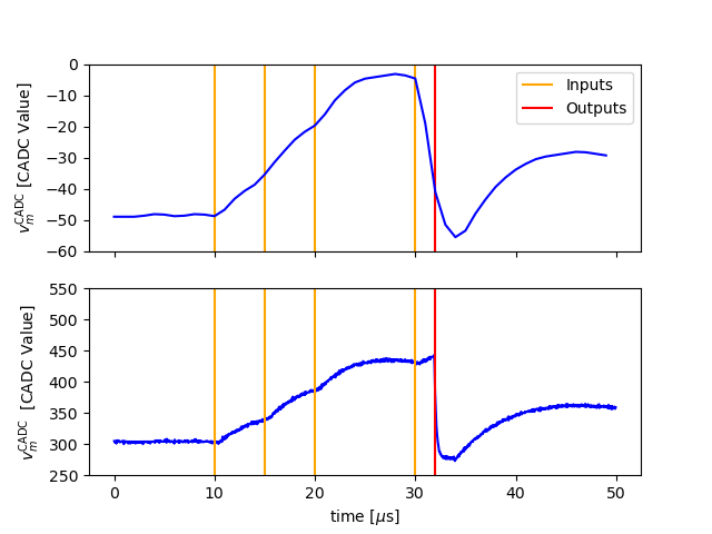
Next we create some input spikes and emulate the network. The membrane potential of the LIF is measured using the columnar ADC (CADC) and the membrane (MADC). While the first allows sampling all neuron potentials on the chip in parallel, the latter can only sample two neurons at the benefit of having a higher temporal resolution. The units are CADC / MADC Values, which in principle are translatable to mV (which will be implemented in the future). When modules are called to infere the networks topology, they return Handles (e.g. g, z) which act as promises to future hardware data which get filled after the hardware experiment is run. Note that in hxtorch the returned hardware data is mapped to a dense time grid of shape (batch_size, time_steps, population_size) of resolution dt.

save_nightly_calibration('spiking_calix-native.pkl')

hxtorch.init_hardware()

# Experiment
exp = hxsnn.Experiment(dt=1e-6)
# To avoid time consuming implict calibration we load a prepared calibration
exp.default_execution_instance.load_calib("spiking_calix-native.pkl")

# Modules
syn = hxsnn.Synapse(
    in_features=1,
    out_features=1,
    experiment=exp)
lif = hxsnn.Neuron(
    size=1,
    experiment=exp,
    enable_cadc_recording=True,
    enable_madc_recording=True,
    enable_spike_recording=True,
    record_neuron_id=0,
    cadc_time_shift=-1)

# Weights on hardware are between -63 to 63
syn.weight.data.fill_(63)

# Some random input spikes
inputs = torch.zeros((50, 1, 1))
inputs[[10, 15, 20, 30]] = 1  # in dt

# Forward
g = syn(hxsnn.NeuronHandle(inputs))
z = lif(g)

print(z.spikes, z.membrane_cadc)

hxsnn.run(exp, 50)  # dt

print(z.spikes.shape, z.membrane_cadc.shape)

# Display
plot_compare_traces(inputs, z)

hxtorch.release_hardware()

Great, we have now seen how easily spiking neural networks are emulated on BSS-2. In order to train them, each layer instance of HXModule has a PyTorch-differentiable numerical representation defined in a member function forward_func. This function allows backpropagating gradients but also to simulate networks. Simulation is enabled by setting mock=True in the Experiment instance:

# Experiment
exp = hxsnn.Experiment(dt=1e-6, mock=True)

# Modules
syn = hxsnn.Synapse(1, 1, exp)
syn.weight.data.fill_(50)  # weights are between -63 to 63
lif = hxsnn.Neuron(1, exp)

# Forward
g = syn(hxsnn.NeuronHandle(inputs))
z = lif(g)

# Simulate
hxsnn.run(exp, 50)  # dt

# Display
plot_mock(inputs, z)

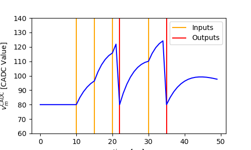
Since the dynamics of the numerics is used to compute gradients it is important to align them to the dynamics of the neurons on hardware. If you compare the y-axes between the first and the second plot you see, that this is not the case here. There are two scalings which can be used to align the dynamics. First there is the trace_scaling which is applied to the measured membrane trace, this allows to scale the hardware values into the expected simulated range. Additionally, the measured traces can be offset either by setting shift_to_fist=True which uses the first measured value as baseline, or setting a trace_offset specifically. The second scaling is the scaling between the weights used in the sofware model and the weights used on hardware, since the “strength” of the weights on BSS-2 depend on the calibration.

First we want to align the membrane ranges. For this, we assume leak=0, reset=0 and threshold=1 for the LIF neuron in the numerics. Neurons can be parameterized with different values for the model in software which is used for gradient computation and the neuron on hardware using a MixedHXModelParameter:

from hxtorch.snn.transforms.weight_transforms import linear_saturating

hxtorch.init_hardware()

# Model parameters
model_threshold = 1.
model_leak = 0.
model_reset = 0.

# BSS-2 parameters
bss2_threshold = 125
bss2_leak = 80
bss2_reset = 80

# Post-processing
# These values are measured in the following
trace_scale = 1.
trace_offset = 0.
weight_scale = 1.


def run(inputs, mock=False, weight_scale=63., trace_offset=0., trace_scale=1., n_runs=10):
    """ """
    traces = []
    for i in range(n_runs):
        # Experiment
        exp = hxsnn.Experiment(dt=1e-6, mock=mock)
        exp.default_execution_instance.load_calib("spiking_calix-native.pkl")

        # Modules
        syn = hxsnn.Synapse(
            in_features=1,
            out_features=1,
            experiment=exp,
            transform=partial(linear_saturating, scale=weight_scale))
        lif = hxsnn.Neuron(
            size=1,
            experiment=exp,
            leak=hxsnn.MixedHXModelParameter(model_leak, bss2_leak),
            reset=hxsnn.MixedHXModelParameter(model_reset, bss2_reset),
            threshold=hxsnn.MixedHXModelParameter(model_threshold, bss2_threshold),
            cadc_time_shift=-1,
            trace_offset=trace_offset,
            trace_scale=trace_scale)
        syn.weight.data.fill_(1.)
        # Forward
        g = syn(hxsnn.NeuronHandle(inputs))
        z = lif(g)
        hxsnn.run(exp, 50)  # dt
        traces.append(z.membrane_cadc.detach().numpy().reshape(-1))
    return traces


# Measure baseline
inputs = torch.zeros((50, 1, 1))
traces = run(inputs)
baselines = np.stack(traces).mean()
print("CADC membrane baseline: ", baselines)


# Measure hardware threshold
# We send a lot input spikes to excite the membrane potential towards the threshold potential
# This will allow us to measure the real threshold value on hardware
inputs = torch.ones((50, 1, 1))
traces = run(inputs, trace_offset=baselines)
bss2_threshold_real = np.stack(traces).max(1).mean()
trace_scale = model_threshold / bss2_threshold_real
print("Leak - Threshold on BSS-2: ", bss2_threshold_real)
print("Trace scaling: ", trace_scale)


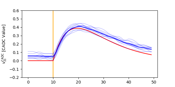
# Next we tune the weight_scaling such that the PSP in the software model and on hardware look the same.
# For this, we send exactly one input to compare the PSPs
weight_scaling = 55.

inputs = torch.zeros((50, 1, 1))
inputs[10] = 1

mock_trace = run(inputs, mock=True, n_runs=1)[0]
bss2_traces = run(inputs, trace_offset=baselines, trace_scale=trace_scale, weight_scale=weight_scaling)

# Display
plot_scaled_trace(inputs, bss2_traces, mock_trace)

hxtorch.release_hardware()

Now that we have aligned the dynamics on hardware and in the numerics, we can use the hardware to emulate out network and use the numerics to compute gradients for a given task. Training networks on BSS-2 using hxtorch.snn works the same as for plain PyTorch. Its easy… sometimes.

In the remainder of this demo we will train a non-spiking leak-integrator (LI) output neuron to resemble a target trace. LI neuron layers are created by using ReadoutNeurons.

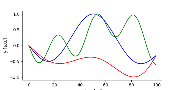
As the target pattern we use a sine:

def get_target(n_out):
    targets = torch.zeros(100, 1, 3)
    for n in range(n_out):
        for i in range(3):
            targets[:, 0, n] += torch.sign(torch.rand(1)-0.5)*torch.sin(
                torch.linspace(0, (2 * torch.pi) / ((0.3 - 2) * torch.rand(1).item() + 2), 100))
    norm = np.abs(targets).max(0)
    return targets / norm.values

targets = get_target(3)

# Display
plot_targets(targets)

import ipywidgets as w

hxtorch.init_hardware()

EPOCHS = 200

exp = hxsnn.Experiment(mock=False)
exp.default_execution_instance.load_calib("spiking_calix-native.pkl")

lin1 = hxsnn.Synapse(128, 3, exp, transform=partial(
            linear_saturating, scale=55))
li = hxsnn.ReadoutNeuron(
    3,
    exp,
    tau_mem=10e-6,
    tau_syn=10e-6,
    leak=hxsnn.MixedHXModelParameter(0., 80.),
    shift_cadc_to_first=True,
    trace_scale=trace_scale,
    trace_offset=baselines)

inputs = (torch.rand((100, 1, 128)) < 0.03).float()

optimizer = torch.optim.Adam(lin1.parameters(), lr=2e-3)
loss_fn = torch.nn.MSELoss()

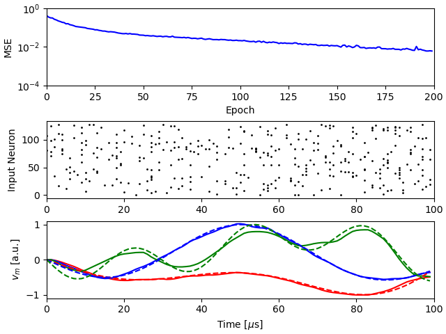
update_plot = plot_training(inputs, targets, EPOCHS)
plt.close()
output = w.Output()
display(output)


for i in range(EPOCHS):
    optimizer.zero_grad()

    # Forward
    g = lin1(hxsnn.NeuronHandle(inputs))
    y = li(g)

    # Run on BSS-2
    hxsnn.run(exp, 100)

    # Optimize
    loss = loss_fn(y.membrane_cadc, targets)
    loss.backward()
    optimizer.step()

    # Plot
    output.clear_output(wait=True)
    with output:
        update_plot(loss.item(), y)

hxtorch.release_hardware()