BrainScaleS-2 on-chip plasticity experiment
In addition to the analog neural network core, BrainScaleS-2 features two embedded general-purpose processors, called PPUs (Plasticity Processing Units). They can be used for experiment control and alterations of configuration during the run-time of an experiment. This example makes use of this feature by show-casing synaptic plasticity.
%matplotlib inline
from os.path import join
import numpy as np
import matplotlib.pyplot as plt
import pynn_brainscales.brainscales2 as pynn
from dlens_vx_v3 import hal, lola, halco, sta
We want to show how the PPUs can be used to rate-code an image in the activity of neurons (our canvas will be the activity of the neurons over time). This is done by switching synapses on and off using a predefined data sequence. Each PPU has 16kiB on-chip memory. For a quadratic image to fit, it is therefore limited to 64x64 pixels. For simplicity, only one of the two PPUs is used.
For loading and converting an image, some helpers are required:
def read_image(path: str) -> np.array:
    """
    Read image from file and scale it to the weight range.
    :param path: Path to image file
    :return: Image data as numpy array normalised to hardware weight range
    """
    image = np.asarray(plt.imread(path))
    # Scale to weight range [0, 63)
    image = image / image.max() * hal.SynapseWeightQuad.Value.max
    return image
Controlling the on-chip plasticity processor
Later, we will define the network topology using the pyNN interface. During the experiment, the PPUs execute an earliest-deadline-first scheduler for tasks to be performed. In PyNN, execution of a plasticity rule is such a task. A plasticity rule is injected via the synapse type of a projection and upon execution is provided with the locations of the synapses in the projection(s) created with this plastic synapse type. The plasticity rule features a method yielding C++-code to be executed as a task on the PPU given the synapse location information. Tasks can be executed periodically, for which a timer object is to be supplied.
For our experiment, we first load an image to be rate-encoded later.

# Read image into 2d numpy array
image = read_image(join("_static", "tutorial", "visions.png"))
Furthermore, we set some environment variables for our microscheduler:
from _static.common.helpers import setup_hardware_client
setup_hardware_client()
The plasticity kernel
We now define the plasticity rule type with the C++-code which imprints the image
onto the spike-trains by alteration of the synaptic weights.
The image data is transferred into a global object image.
The entry point of the plastic task is called PLASTICITY_RULE_KERNEL
and is supplied with synapse location information corresponding the the projection
in PyNN. Within the task function, the program writes synapse weight values
row-wise via set_weights(weight_row, row).
Since the task is scheduled periodically configured via the Timer object, after
each write, the period duration is waited before the next row of the image is written.
Over time, this leads to each row of the image being present and imprinting itself
onto the neurons’ firing rate.
import textwrap

class PlasticityRule(pynn.PlasticityRule):
    def __init__(self, timer: pynn.Timer, image: np.array):
        """
        Initialize plastic synapse with execution timing information,
        the image pixels and initial weight.
        """
        pynn.PlasticityRule.__init__(self, timer)
        self.image = image
        assert self.timer.num_periods == len(self.image)

    def generate_kernel(self) -> str:
        """
        Generate plasticity rule kernel to be compiled into PPU program.

        :return: PPU-code of plasticity-rule kernel as string.
        """
        return textwrap.dedent("""
        #include "grenade/vx/ppu/synapse_array_view_handle.h"
        #include "grenade/vx/ppu/neuron_view_handle.h"
        #include "libnux/vx/dls.h"
        #include <array>

        using namespace grenade::vx::ppu;
        using namespace libnux::vx;

        /**
         * PPU currently executing this code (top/bottom).
         */
        extern volatile PPUOnDLS ppu;

        /**
         * Image data.
         */
        uint8_t const image[{image_h}][{image_w}] = {{
            {image_pixels}
        }};

        /**
         * Currently to be presented row in image.
         */
        uint32_t current_row = 0;

        void PLASTICITY_RULE_KERNEL(
            std::array<SynapseArrayViewHandle, 1>& synapses,
            std::array<NeuronViewHandle, 0>&)
        {{
            // only update weights when code is executed on the correct PPU
            if (synapses[0].hemisphere != ppu) {{
                return;
            }}
            for (size_t row = 0; row < synapses[0].rows.size(); ++row) {{
                // load new vertical line of image
                vector_row_t weight_row;
                size_t w = 0;
                for (auto const column: synapses[0].columns) {{
                    weight_row[column] = image[w][current_row];
                    w++;
                }}

                // alter weights in synapse memory
                synapses[0].set_weights(weight_row, row);
            }}
            current_row++;
        }}
        """.format(image_h=len(self.image), image_w=len(self.image[0]),
                   image_pixels=",".join(["{" + ", ".join(
                       [str(int(pixel)) for pixel in row]) + "}"
                            for row in self.image])))
The experiment
For this simple binary on-off plasticity, we don’t need the full-fledged capabilities of the neurons and therefore configure them to bypass-mode, where every incoming spike elicits an output spike.
pynn.setup(enable_neuron_bypass=True)
Our network uses a single-layer feed-forward structure. External Poisson stimulus is generated with a constant rate. We use multiple sources for decorrelation of the neurons’ spikes in order to prevent congestion effects due to the neuron bypass mode.
bg_props = dict(
    start=0,  # ms
    rate=4000,  # Hz
    duration=64  # ms
)
external_input = pynn.Population(64, pynn.cells.SpikeSourcePoisson(**bg_props))
The target population consists of 64 neurons, spikes are recorded.
neurons = pynn.Population(64, pynn.cells.HXNeuron())
neurons.record(["spikes"])
Since the external stimulus population’s size matches the internal population’s size, a one-to-one connector is used as projection. Initially the weight is set to zero, the PPU will alter it during the experiment.
timer = pynn.Timer(
    start=0., # ms
    period=1., # ms
    num_periods=len(image))
plasticity_rule = PlasticityRule(timer=timer, image=image)
synapse = pynn.standardmodels.synapses.PlasticSynapse(
    plasticity_rule=plasticity_rule, weight=0)
pynn.Projection(external_input,
                neurons,
                pynn.OneToOneConnector(),
                synapse_type=synapse)
We run the experiment for 64 ms, during which we expect a weight change every ms leading to all image columns being present as weights for this duration one after the other.
pynn.run(64) # ms
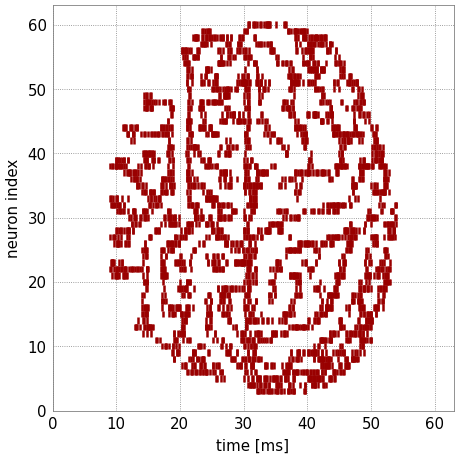
Last, the recorded spike-trains are visualized.
spikes = neurons.get_data("spikes").segments[0]
spiketrains = []
for spiketrain in spikes.spiketrains:
    spiketrains.append(spiketrain.base)

fig = plt.gcf()
fig.set_size_inches(4, 4)

plt.eventplot(spiketrains, color='#990000')
plt.xlim(0,64)
plt.ylim(0,63)
plt.xlabel("time [ms]")
plt.ylabel("neuron index")
fig.show()
# assert spikes are recorded
total_spikes = np.sum([len(spikes) for spikes in spiketrains])
assert total_spikes > 0, "No spikes recorded"
We see a replicated version of the original image encoded in the time evolution of the neurons’ firing rates.
