Exploring the dynamic range

In this example we’ll explore the dynamic range of synaptic stimulation.

We will

set up a network using PyNN
incrementally add more and more synaptic stimulation
quantify the effect of the synaptic stimulation on the membrane of different neurons for excitatory and inhibitory stimulation

In order to use the microscheduler we have to set some environment variables first:

from _static.common.helpers import setup_hardware_client
setup_hardware_client()

We’ll also configure matplotlib and import some tools.

%matplotlib inline
import numpy as np
import pandas as pd
import itertools
import matplotlib.pyplot as plt
from contextlib import suppress
with suppress(IOError):
    plt.style.use("_static/matplotlibrc")

import pynn_brainscales.brainscales2 as pynn

Before we define our network, we load the default calibration.

A default calibration is generated for every setup every night. We save the nightly calibration in two variables such that we can use it later when we define our neuronal network.

from _static.common.helpers import get_nightly_calibration
calib = get_nightly_calibration()

Define network in PyNN

First, we will set up some variables determining the sweep we want to perform.

neurons = range(0, 512, 64)
weights = range(0, 300, 32)
receptor_types = ["inhibitory", "excitatory"]

We will store the results in a dictionary.

from collections import defaultdict
results = defaultdict(list)

We configure the logger to print some output during the run.

log = pynn.logger.get("dynamic_range")
pynn.logger.set_loglevel(log, pynn.logger.LogLevel.INFO)

Next we run the network multiple times with various configurations.

from dlens_vx_v3 import hxcomm

# to speed things up, we keep the connection alive between experiments
with hxcomm.ManagedConnection() as connection:

    for neuron, receptor_type in itertools.product(neurons, receptor_types):

        # the neuronPerm
        pynn.setup(connection=connection,
                   neuronPermutation=[neuron],
                   initial_config=calib)

        # always have only 1 neuron
        number_of_neurons = 1

        population = pynn.Population(number_of_neurons,
                                     pynn.cells.HXNeuron())

        # disable spiking
        population.set(threshold_enable=False)

        # record the membrane voltage
        population.record("v")


        input_spiketimes = [0.5]
        stimulus = pynn.Population(1,
                                   pynn.cells.SpikeSourceArray(spike_times=input_spiketimes))
        proj = pynn.Projection(stimulus,
                               population,
                               pynn.AllToAllConnector(),
                               receptor_type=receptor_type,
                               synapse_type=pynn.standardmodels.synapses.StaticSynapse(weight=0))

        # Adjust weights of existing projections and add new projections if the desired weight
        # exceeds the maximum weight which can currently be implemented.
        for w in weights:

            sign = 1 if receptor_type == "excitatory" else -1

            proj.set(weight=sign * w)

            pynn.run(1) # ms (hw)
            membrane = population.get_data().segments[-1].irregularlysampledsignals[0]

            min_membrane = float(membrane.min())
            max_membrane = float(membrane.max())

            results["weight"].append(w)
            results["receptor_type"].append(receptor_type)
            results["neuron"].append(neuron)
            results["membrane_min"].append(min_membrane)
            results["membrane_max"].append(max_membrane)

            log.info(f"{neuron=} {receptor_type=} {w=} "
                     f"{min_membrane=} {max_membrane=}")

            pynn.reset()

        pynn.end()

    log.info("experiment done")

    df = pd.DataFrame.from_dict(results)

    log.info("DataFrame created")

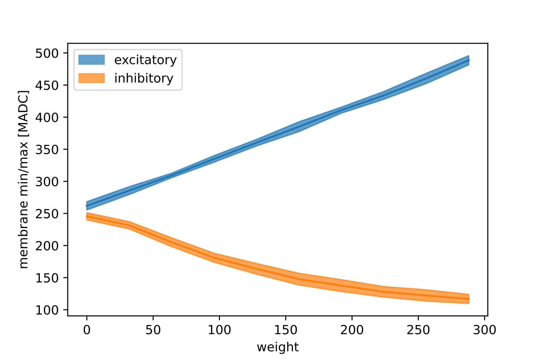
Now, all results are stored in the Pandas DataFrame that we can analyse with the code below. For the excitatory stimulation we plot the mean of the maximum of the membrane trace and the variance over the neurons. We do the same for the inhibitory stimulation but take the minimum of the membrane trace this time.

First we aggregate over the neurons and create convience columns for the analysis:

def aggregate(df):
    return (df
            .groupby(['receptor_type', 'weight'])
            .agg(**{f"{method}_{col}" : (col, method) for col, method
                               in itertools.product(["membrane_min", "membrane_max"],
                                                    ['mean', 'std'])})
            .reset_index()
    )
df_agg = aggregate(df)

Next we define a helper function to plot the variance over the neurons as an error band:

def plot_with_errorband(ax, x, y, error, label, color):
    ax.plot(x, y, '-', color=color)
    ax.fill_between(x, y-error, y+error, label=label, color=color, alpha=0.7)

Now we can do the final plot:

fig, ax = plt.subplots()

lookup = {'excitatory_color' : "tab:blue",
          'inhibitory_color' : "tab:orange",
          'excitatory_column' : "membrane_max",
          'inhibitory_column' : "membrane_min"}

for receptor_type in ['excitatory', 'inhibitory']:

    df_ = df_agg[df_agg.receptor_type==receptor_type]

    color = lookup[f"{receptor_type}_color"]
    column = lookup[f"{receptor_type}_column"]

    plot_with_errorband(ax=ax,
                        x=df_["weight"],
                        y=df_[f"mean_{column}"],
                        error=df_[f"std_{column}"],
                        label=receptor_type,
                        color=color)


ax.set_xlabel("weight")
ax.set_ylabel("membrane min/max [MADC]")
ax.legend()